How Many Samples to Collect? Sample Till You’re Sure Part 2

Welcome to the second and final part of our in-depth blog series: How Many Samples to Collect? Sample Till You’re Sure.

Gus Manning, Chief Technical Officer & company founder, has made it his life’s work to bring accurate, cost-effective, and easy-to-use samplers to the workplace and make work environments safer for workers. The OSHA enforcement strategy – assuming workplace exposures could be well characterized by a small number of samples – has been found deficient in a number of classic studies, cited in this series.

How Many Samples to Collect (Part 2)

(Workplace Variation Was Greater Than We Thought)

Part 1 of this discussion revealed that variation in workplace exposures is typically greater than many IH’s had thought. High workplace variation arising from lognormal exposure distributions led the IH community to generally underestimate workplace exposures. The IH Data Analyst, provided free by AIHA, allows an IH to enter real data and classify an exposure group as to its likelihood of compliance with a PEL or an OEL. This allows an IH to “sample till you’re sure”. In this Part 2, we explore the background issues more deeply.

Worker Exposure Categories

As part of the overall system provided by AIHA’s Improving Exposure Judgments initiative, exposure range are classified into 5 Exposure Bands, relative to a selected OEL, as follows

The IHDA (IH Data Analyst) works with the Table above. Given a population of personal exposure sample results, IHDA provides a graphical output to inform the user of the following:

1. The degree of fit (agreement) with the (lognormal) statistical model
2. The Probability that the 95th percentile exposure is within each of bands 0, 1, 2, 3, and 4.
3. Other useful Information

Your Intuition May Initially Disagree with IHDA Results

During initial use of the AIHA’s IH Data Analyst, many IH practitioners found that IHDA placed their exposures in a higher Exposure Band than they would have guessed from intuition or from “normal” statistics. Studies by the AIHA Exposure Assessment Committee showed that IH practitioners tend to underestimate exposures after inspecting data from a few exposure tests.

There are important reasons for this, as follows:

1. Exposure data tend to be more variable than we would expect.
2. Exposure data tend to follow a skewed (lognormal) rather than a normal statistical pattern.

Workplace Variation Tends to be Greater Than We Thought

In Part 1, we mentioned OSHA’s policy that 100% of exposures must be below the PEL. In practice, OSHA ignores employers’ exposure data, relying on its rare sampling visits to detect overexposures. This policy would work if workplace exposures were uniform and constant, but they are NOT. When workplace exposures are variable, replicate samplings often yield different results.

While a few tests may give values below the PEL/OEL, a proper statistical analysis will often predict a higher-than-expected range of exposures arising from the lognormal (skewed) nature of data. The variable and skewed nature of workplace exposures has led many IH practitioners (and OSHA) to underestimate exposure risks as discussed in the following paragraphs.

Uniform Exposures and “Homogeneous Exposure Groups” in the Past

Prior to the publications of Rappaport (1,2) and Nicas (3) many in the IH community assumed workplace exposures were uniform, and only a few tests would be required to assess workplace exposures. Following OSHA’s approach, IH practitioners believed the accuracy of sampling methods was a more important issue than the variation in workplace chemical exposure.

Researchers Discover Workplace Variation

A belief in uniform exposures in the 1980s led to common use of the term HEG (Homogeneous Exposure Group), referring to a group of workers doing similar jobs in the same location, who were expected to have the same (homogeneous) exposures. Early in the 1990s, Professor Steven Rappaport (1) surveyed more 15,295 on 183 HEGs exposure measurements, finding that HEGs were not usually ”homogeneous”, as previously believed.

Following Professor Rappaport’s (1,2) disclosures, the term HEG was scrapped in favor of SEG (Similar Exposure Group), an admission of greater-than-expected variations within worker groups.

Subsequently, Professor Nicas (3) compared workplace variation with analytical variation saying:

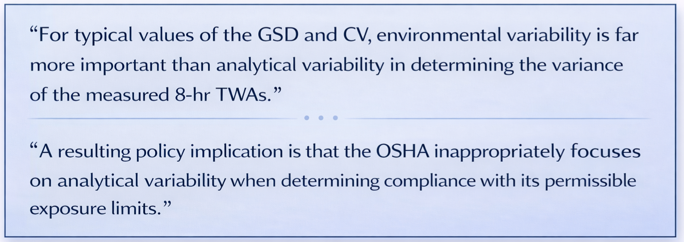
More recently, Mulhausen, Hewett, et al. (4) confirmed Rappaport’s and Nicas’s view.

GSD (Geometric Standard Deviation)

GSD is used to express variation in workplace exposure data which usually show a (skewed) lognormal pattern rather than a normal (Gaussian) pattern. GSD numbers are actually logarithms. A GSD of 2.0 means the 67th percentile exposure is two logarithms (100 times) greater than the 33rd percentile exposure. Further, a GSD of 4.0 indicates a variation that is 100 times that of GSD = 2.0.

When the AIHA IHDA says that typical workplaces have GSD between 1.5-4.0, they are saying that some “typical” workplaces (with GSD = 4.0) have variation that is more than 100 times greater than other “typical” workplaces. Even in a “low variation” workplace (with GSD = 1.5), the 67th percentile exposure would be 32 times as great as the 33rd percentile exposure.

Skewed or Lognormal Data Distribution in Workplace Data

Statisticians call data “normal” if the range of higher values versus lower values are symmetrical around the mean (average), the so-called “normal” “bell-shaped curve” (below, left). Typical workplace data have been found to yield skewed data that are not symmetrical around the mean. Rather, the data higher than the mean includes a much larger range of high values, while the range of values below the mean is much smaller. This is illustrated in the graphic plot below (below, right).

Random variations tend to produce “normal” data. Skewed data arise when there are more causes that lead to higher results, and fewer causes that leads to lower results. The most common environmental contamination events tend to be leaks and spills which lead to higher values. There are fewer causes that leads to lower values, hence, workplace exposure data tend to be “skewed high”  leading to a much greater range in the high values than in the lower values.  This is true, and it agrees with common sense.

Why Skewed, Lognormal Results Lead to Errors in IH Professional Judgment

When you analyze only a few samples, you are most likely to get the “most probable” values, i.e., values that are near to the peak (most probable) value.

In the plot (right), you can see the most probable value is 1.5, the 5th percentile value is 0.8, and the 95th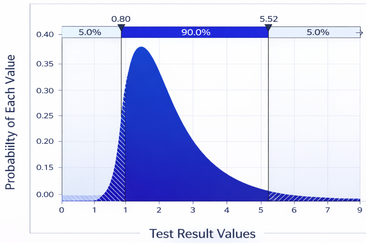 percentile value is 5.5. Thus, the 5th percentile value is only 0.7 points lower than the peak (most probable) value, while the 95th percentile is 4.0 points higher than the peak (most probable) value.

Intuition usually tells you that the higher range (above the ave.) should be similar to the low variation (below the ave.) but in a skewed distribution this is not true, and intuition will fail you.

Bayesian Statistics

The AIHA IHDA utilizes Bayesian statistics, a novel method for analyzing skewed data that incorporates prior knowledge of a system in its calculations. A detailed explanation of Bayesian statistics is beyond the scope of this article, but we reference an accessible treatment (5). With IHDA, AIHA has provided a tool that addresses the problem of Improving Exposure Judgments and provides a higher Standard of Care than mere regulatory compliance (not getting caught).

REFERENCES

(1)S. M. Rappaport, H. Kromhouta & E. Symanski (1993) VARIATION OF EXPOSURE BETWEEN WORKERS IN HOMOGENEOUS EXPOSURE GROUPS, American Industrial Hygiene Association Journal, 54:11, 654- 662, DOI: 10.1080/15298669391355198

(2) Selection of the Measures of Exposure for Epidemiology Studies S. M. Rappaport Pages 448-457; https://doi.org/10.1080/1047322X.1991.10387912

(3) Nicas, M., Simmons, B. P., & Spear, R. C. (1991). ENVIRONMENTAL VERSUS ANALYTICAL VARIABILITY IN EXPOSURE MEASUREMENTS. American Industrial Hygiene Association Journal, 52(12), 553–557. https://doi.org/10.1080/15298669191365199

(4) https://www.aiha.org/education/elearning/online-courses/making-accurate-exposure-risk-decisions

(5) Everything is Predictable – How Bayesian Statistics Explain Our World, Tom Chivers, Atria (2024)

APPENDIX A – Free Tools Provided by AIHA

Making Accurate Exposure Risk Decisions | AIHA

IHDA-AIHA Tool Download | AIHA

APPENDIX B – Occupational Exposure Limits (OELs)

American Conference on Government Industrial Hygienists (ACGIH) – Threshold Limit Value (TLV)

National Institute for Occupational Safety and Health (NIOSH) – Recommended Exposure Limit (REL)

Occupational Safety and health Administration (OSHA) – Permissible Exposure Limit (PEL)

OSHA – Short Term Exposure Limit (STEL) & OSHA Ceiling Limit

In addition to these organizations, the US Environmental Protection Agency (USEPA), foreign governments, as well as companies and private organizations are active is setting OELs or ELs. The fact that many organizations have set different OELs for the same chemical substance reflects the fact that there is disagreement about what is a “Safe Exposure Level”. In principle, any and all OELs are meant to describe a Limit below which is worker will suffer no harm if exposed at or below the OEL during an entire working life.

As guidance, we can say that selecting a lower OEL will likely reduce risk. An industrial hygiene manager must use professional judgment and select an OEL for his/her practice.